The Clean Water Act contains provisions that prohibit the discharge of eight chemicals. These regulations require specific pollutants to be absent or exist at extremely low concentrations. To be able to work with agencies charged with the enforcement of these regulations, the metal-finishing industry needs to understand the concept, definition, and use of the limit of detection (LOD).
This provides an opening for many regulatory schemes based on perception versus fact.
The concept of LOD is a very important and unusual issue in environmental regulation because it moves the work of the analytical laboratory below the level of quantitation and into an imprecise area where an analyte can be detected, but the exact amount of that analyte cannot be precisely measured. This provides an opening for many regulatory schemes based on perception versus fact. Analytes measured at detection are generally reported in the parts-per-billion (ppb) or parts-per-trillion (ppt) range in complex matrices. This low-level detection in itself presents unique difficulties for the analytical laboratory. In addition, LOD is a confusing concept because there are many definitions of it, and many of these have been misused and intermingled. This has caused unnecessary difficulties in creating environmental statutes, interpreting the legislation, and equitably enforcing the laws. Semantics can further complicate matters in that zero discharge is sometimes used in place of LOD terminology, or the terms are used interchangeably.
Three major agencies provide direction and definition in detection-limit discourse. They are the American Chemical Society (ACS), the International Union of Pure and Applied Chemistry (IUPAC), and the United States Environmental Protection Agency (EPA). The definitions of LOD, the limit of quantitation (LOQ), method detection limit (MDL), and practical quantitation limit (PQL), and the basis and intended use of each methodology are presented and analyzed in this article.
IUPAC/ACS Methodology
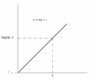
Fig. 1: Analytical calibration curve of signal versus concentration c.
As a response to the confusion that existed both in academia and in the chemical literature with regard to numerous conflicting data on detection limits, the IUPAC adopted a model for these calculations in 1975.1 The ACS Subcommittee on Environmental Analytical Chemistry reaffirmed this standard in 1980.2 The IUPAC definition of 1975 states the following:
The limit of detection expressed as a concentration, cL, is derived from the smallest signal, xL that can be detected with reasonable certainty for a given analytical procedure.1
However, analysts have been slow to adopt the IUPAC/ACS methodology, and this has necessitated additional symposia and committee reports to reaffirm the preferred method for determining the detection limit.3.4
The LOD is a statistical concept that is intended to reflect the magnitude of unavoidable random fluctuations in measurements at low analyte concentrations. The detection limit of an analytical procedure is a number expressed as the lowest concentration of an analyte that can be distinguished with reasonable statistical confidence from a field blank. The blank is a hypothetical sample containing zero concentration of the analyte.
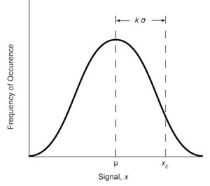
Fig. 2: Normal distribution curve for a measured variable x with standard deviation σ and mean μ.
The entire ACS procedure is based on blank measurements and the calculation of the standard deviation of those measurements. The blank used most often is reagent-grade water or a solvent of interest that is both reproducible and controllable. The detection limit is estimated from the response or signal of an instrument to the blank but is usually reported in terms of concentration or mass. The conversion of the signal output to concentration limits is accomplished with the analytical calibration curve. Most analytical methods require the construction of an analytical calibration curve for the determination of unknowns. The relationship between signal and concentration is provided by the calibration curve shown in Figure 1.
The analytical calibration relationship can be expressed as
x=mc+i (1)
where m is the slope or analytical sensitivity, and i is the intercept. The functionality between x and c can be obtained by performing a linear regression analysis on the data, which generates the calibration curve. The ability to solve accurately for concentration c is dependent on how well the sensitivity and intercept are known. When the calibration curve is obtained in the linear response region of the method, and the number of data points used in the construction of the calibration curve is maximized, the values of m and i will be better defined.
The amount of error associated with a measurement of signal x can be statistically estimated. If a large number of observations are made, and the results are plotted versus the frequency of occurrences, a normal error curve will result. The population mean value of the response µoccurs at the center of the Gaussian curve, which is symmetrical about the mean. The population standard deviation O’ defines the width of the curve from the mean. The curve is shown in Figure 2 and is given by the formula
y = (1/σ √2π x exp -[(x – µ)2/2σ2] (2)
For an infinite set of data, the curve is characterized by the mean and standard deviation. For a finite set of data, µ and cr are approximated by the arithmetic mean x, and the standard deviation S. These two variables are given by the following formulas:
x– = Σixi/n (3)
S = [Σi(xi – x–)2]1/2 / (n – 1) (4)
where n is the total number of finite data points.
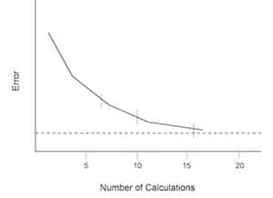
Fig. 3: Error versus replicate calculations in an analytic procedure.
Because this curve includes-all values of x, the area under the curve can be expressed in terms of the probability that a measured value would fall somewhere under the curve. The relationship between area and probability can be measured to estimate the chance that a newly measured x value xE would be a certain number of standard deviation units away from the mean response.
The specifics of the ACS methodology for the calculation of LOD will be useful in further explaining the relationship of the normal distribution of data with calibration curves that the data generated. The ACS LOD is calculated as follows:
- A statistically significant number of measurements of the blank sample containing a zero concentration of analyte are made. At least 10 and up to 20 replicates are needed for sufficient accuracy in standard deviation calculations.3 The blanks should be treated exactly like samples and should be passed through the entire analytical procedure. Sixteen measurements are generally selected to minimize the rate of change of the error introduced in the calculations. This can be shown graphically in Figure 3.6
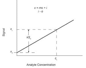
Fig. 4: Analytical calibration curve with limiting concentration cL determined to be statistically different from mean of blank measurements xb by kSb.
- The standard deviation of the 16 blanks, Sb, is calculated using Eqs. (3) and (4). (The units of the standard deviation are units of signal, not concentration.)
- Five solutions of varying analyte concentrations in the solvent of the blank are made. These solutions are run by the methodology of choice, the data collected, and the analytical calibration curve of signal x versus concentration c constructed using linear regression.
- The LOD in units of concentration is calculated from the derived slope of the calibration curve and the calculated Sbin units of the signal. By definition,
xL = x–b + kSb (5)
where xL is the smallest discernible analytical signal, xb is the average signal from replicate blank determinations, and k is a numerical factor chosen in accordance with the desired confidence level. This is shown graphically in Figure 4.
The concentration cL, which corresponds to the smallest discernable analytical signal xL, is written as
cL = (xL – x–b)/m (6)
Because the mean blank reading xb, is not always 0, the signal must be background corrected (xL – xb). By substituting Eq. (5) with Eq. (6),
cL = kSb/m (7)
If k = 3 (three standard deviation units), which allows for a confidence level of 99.86%, then the signal developed by the analyte will be very much larger than the average signal calculated from replicate blank determinations; then,
cL = 3Sb/m = LOD (8)
and cL is a true reflection of the LOD when m is well-defined, and i is essentially zero. Equation (8) is the ACS definition of LOD. The selection of three standard deviation units (k = 3) is the choice of the ACS to ensure that the smallest discernible analytical signal xL can be measured and is not caused by random fluctuations of the blank signal.
The key features of ACS LOD analysis are multiple replicate blanks; blank measurement devoid of analyte; reproducible blanks; a noniterative process; and a calibration curve required to calculate the slope and thus derive the LOD.
There are other approaches to calculating cL values that are similar to the IUPAC/ACS model in that Sb and k factors are involved; however, some authors have recommended other values of k, which significantly alters the resultant value of cL.7 Thus, when other limiting concentrations are reported as the detection limit, but the confidence level k is different, confusion obviously results. It is for this reason that the IUPAC and ACS have recommended that xL be reported in all literature using their k value, xL (k = 3). It would be very helpful to add the next logical step and include the k values when cL values are reported: cL (k = 3).5
Another source of confusion in the literature, compounding the LOD anomalies, is the use of multiple standard deviations. The standard deviation of the mean, standard error of the mean,8 the pooled standard deviation of the mean (Sp),9,10 or the relative standard deviation (RSD)9,11 have all been used by various authors. Each of these standard deviation expressions is important and has its place in analytical chemistry; however, the use of these expressions in calculating cL may result in significant deviations from the IUPAC/ACS model and further complicate the reporting of a consistent LOD.
Limit Of Quantitation
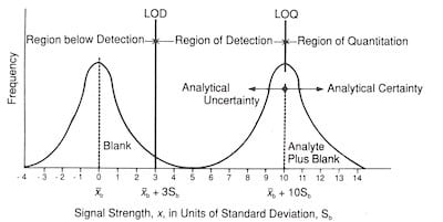
Fig. 5: Relationship of LOD and LOQ to signal strength.
The LOD is designed to statistically separate the blank measurement signals from the true analyte signals. As such, it is an analytical concept that provides information with regard to the detect/no-detect decisions. It is not a value that has quantitative analytical significance. Several authors have recognized the need to define a “minimum working concentration,” which is an elevated concentration of analyte that provides analytical certainty of quantitation.2,12 The idea behind these higher limits is that the analyte can be determined with a reasonable degree of precision when present at levels significantly above its LOD.
When the analyte concentration increases as the analyte signal increase above its smallest detectable signal xL a minimum criterion representing the ability to quantify the sample can be established reasonably far away from the average signal calculated from replicate analyses of the blank, xb. This criterion is called the limit of quantitation (LOQ).
For LOD work, LOQ is defined by the ACS as 10 standard deviations away from the xb.2 Samples that are measured having a signal x, where x > 10Sb, are said to be in the region of quantitation. Samples having a signal x, where 10Sb > x > 3Sb, are said to be in the region of detection. Samples having a signal x, where x > 3Sb, are not detectable. This may be shown graphically, as in Figure 5.
Method Detection Limit
In the real world, the requirement to calculate a detection limit based on a field blank presents an enormous problem. The chemical background in which regulated pollutants exist is most often complex. The matrices that provide the background for practical detection-limit work are commonly municipal sewerage, effluent from complex industrial operations, the outfall from domestic sources with its bewildering array of consumer products, and land run-off. To create a blank that duplicates such matrices and that could be used with the ACS LOD methodology (devoid of analyte) is a chemical problem of enormous proportions. For pragmatic reasons, therefore, a detection-limit procedure was developed that focuses on an operational definition of the detection limit. This procedure, adopted by the EPA, is the method detection limit (MDL).8,13
The MDL is a procedure whereby the LOD is established with the analyte of concern in a complex matrix. The procedure establishes a relationship between detectability and analytical precision (i.e., an indicator of the reproductibility of a determination).
This method is very different from the ACS methodology, where the chemistry of the blank in a relatively simple or reproducible matrix is used as the basis for detection. The MDL refers to samples processed through all of the steps comprising an established analytical procedure. The emphasis in the MDL approach is on the operational characteristics of the definition. The MDL is considered meaningful only when the method is in the detect mode (i.e., the analyte must be present).8
The EPA defines the MDL as follows:
The minimum concentration of a substance that can be measured and reported with 99% confidence that the analyte concentration is greater than zero and is determined from replicate analysis of a sample in a given matrix containing the analyte.13
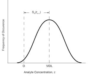
Fig. 6: MDL depicted as an error distribution, where S(tn-1) is selected for 99% confidence that MDL is greater than zero.13
The MDL can be presented as an error distribution. The definition of MDL implies that, on average, 99% of the trials measuring the analyte concentration at the MDL must be significantly different from zero analyte concentration. The assumptions implicit in the methodology are that the error distribution associated with the analytical measurement has a homogeneous variance, is normally distributed, and that the variability as measured by the standard deviation is a function of the concentration being measured. The exact mathematical definition of MDL is
MDL= S(tn-1) (9)
where S is the standard deviation of all replicate measurements of analyte in the matrix of interest and is defined as in Eq. (4); and (tn-1) is the student’s t-test distributions for 99% confidence level for n-1 degrees of freedom. This can be depicted graphically, as in Figure 6.
The exact methodology for MDL determination has been described elsewhere.8,13 It is a method that establishes a relationship between detectability and analytical precision based on an iterative process for analyzing the analyte in a given matrix. It is a procedure that was developed for applicability to a wide variety of physical and chemical methods, including reagent-grade water as the analyte or matrix change; It requires a complete and well-defined analytical method. Because the MDL will vary as the analyte or matrix changes, it is site-specific.
To determine the MDL, the analyst must prepare at least seven aliquots of sample that may have been spiked from one to five times an estimated MDL level (knowledge of the analyst and methodology is key to this parameter). The final calculated MDL of the replicate analyses is then compared with the original estimate to determine its reasonableness. If the result fails, the iteration begins again with a new estimate of MDL.
The specifics of the EPA methodology for the MDL calculation will be useful in explaining the relationship between operational data and the LOD. The MDL procedure is summarized as follows:
- Make an·estimate of the detection limit. This estimate is dependent on the experience of the analyst. It is based on any of the following estimates: 2.5-5.0 times the instrument signal-to-noise ratio; three times the standard deviation of replicate analyses of the analyte in reagent-grade water; that region of the standard calibration curve that exhibits a significant change of sensitivity; or instrumental limitations.
- Analyze the sample in the matrix of interest. If the result is less than the estimated level (i.e., no detect), spike the unknown with analyte to bring the level of analyte between one and five times the estimated detection limit. If the sample result is within one to five times the estimated detection limit, proceed to step 3. If the sample is greater than five times the estimated detection limit, there are two options: obtain a sample with a lower level of analyte; or the sample may be used if the analyte level is not greater than 10 times the MDL of the analyte in reagent-grade water. The variance of the analytical method changes as the concentration changes. Therefore, as the concentration moves away from lower levels, the MDL may not truly reflect the variance at lower analyte levels.
- Take a minimum of seven aliquots of the sample and analyze it through the entire analytical procedure. If a blank measurement is required by the analytical procedure, obtain a separate blank for each sample aliquot.
- Calculate the standard deviation S [as in Eq. (4)] and variance S2as follows:
S2 = Σin(xix–)2/(n – 1) (10)
- Compute the MDL as in Eq. (9).
- If the calculated MDL is within one to five times the estimated MDL, then the value is the detection limit for that procedure in the matrix of interest. Compute the 95% confidence interval estimates for the MDL. The lower confidence limit equals (0.64)(MDL), and the upper confidence limit equals (2.20) (MDL). These confidence limits are derived from percentiles of the chi-square distribution (a nonnormal distribution).
- If the calculated MDL is not within one to five times the estimated MDL, use this calculated value as a new estimate of MDL. Spike the analyte into seven new aliquots at the level of the estimated MDL and proceed with steps 3-6. If this second calculated value is within one to five times the estimated MDL, then the procedure is complete. If not, use the second calculated MDL as the estimate for the next iteration of the detection limit. The iterations continue until the calculated MDL falls within one to five times the estimated MDL.
- When the detection limit is calculated, a new aliquot is spiked at one to two times the calculated MDL. This sample is run through the analytical procedure, and the percent recovery· is calculated. A recovery of greater than 75% is generally accepted as evidence of a useable MDL.
There are limitations to the MDL procedure that must be recognized so that analysts, engineers, and regulators can understand the basis of the methodologies they are using in regulations. These limitations are the following:
- The basic assumption of MDL that precision is indicative of detectability may not always be applicable.
- The procedure does not take into account the effects of poor accuracy (bias). It is possible to be very precise without being accurate.
- Precision is not entirely independent of concentration; the concentrations chosen for an MDL study can make a difference in the MDLs obtained.
- The procedure warns that it may be necessary to determine a lower concentration of analyte that will result in a lower MDL but provides only limited help in estimating this lower level via the two aliquot processes and reestimating the MDL.
- The most significant objection to MDLs is one for which the procedure is not to be blamed. Most laboratories tend to perform MDL determinations with replicates in reagent-grade water, thus disregarding the effect of complex matrix components. When the MDL is determined under these conditions, the value obtained is one that can only be considered achievable by the laboratory under the most favorable circumstances. It is the detection limit of the “perfect sample.”14These MDLs are used by individual laboratories to determine the laboratory-specific minimum detection capabilities. Laboratories have an obligation to identify that these idealized detection limits are performed on reagent-grade water.
The EPA has derived and published MDLs for a number of methods and substances in reagent-grade water, but it acknowledges that those values will vary depending on both instrument sensitivity and matrix effects.15,17 As such, it states that these published “idealized” MDLs should never be used as a basis for setting regulatory compliance.18 Several authors and members of the regulated community have expressed concern and frustration with the use of MDL values obtained under ideal situations as the basis of regulation and their no achievability in real-world matrices.19-21 It is important to realize that these limits are not to be used as the basis of regulation. Some value greater than those must be selected so as to account for interference incumbent in complex matrices.
An additional, equally important reason for not using these MDLs is the question of false positives. By definition of the MDL, there is a 1% chance that a measurement of effluent will be greater than the MDL. That is if 100 measurements are made on blanks that are devoid of analyte, then one detect is expected. There is a statistical variability on the 100 measurements in that there may be no detect or two or more.
The chance of getting no detects from 100 observations is 0.99100 = 0.36, or 36%. The complementary probability of getting at least one detect is 100 – 36 = 64%. Thus, there is a–64% probability that the blank effluent will be declared in violation by the time 100 tests have been made on the effluent.22 The risk of being declared in violation when in fact, the effluent is in compliance associated with a set of 100 samples is 64%. As the sample size increases, the discharge risk also increases and approaches 100%. What this means is that eventually, even blank effluent will be declared in violation. It is only a matter of time and number of samples collected!
Practical Quantitation Limit
The MDL is matrix, laboratory, instrument, and analyst (for certain methodologies) specific.18,23 As such, it does not provide a useful measure of LOD that allows qualified laboratories to communicate with each other. The MDL is not a measure of an analyte that has quantitative significance. It is a litmus test of detection, not quantitation. Because of the need to provide a more workable detection limit method between laboratories, the EPA has defined a practical quantitation level (PQL). The EPA defines this term as follows:
The lowest level that can be reliably achieved within specified limits of precision and accuracy during routine laboratory operating conditions is the Practical Quantitation Level (PQL). The PQL thus represents the lowest level achievable by good laboratories within specified limits during routine laboratory operating conditions. The PQL is determined through interlaboratory studies. Differences between MDLs and PQLs are expected since the MDL represents the lowest achievable level under ideal laboratory conditions, whereas the PQL represents the lowest achievable level under practical and routine laboratory conditions.
If data are unavailable from interlaboratory studies, PQLs are estimated based on the MDL and an estimate of a higher level, which would represent a practical and routinely achievable level with relatively good certainty that the reported value is reliable.24
The basis for setting PQLs is quantitation; precision and accuracy; normal operations of a laboratory; and the fundamental need in a compliance monitoring program to have a sufficient number of laboratories available to conduct analyses. The PQL is analogous to the LOQ as defined by the ACS in that both define the concentration of an analyte above, which is the region of quantitation, and below, which is the region of less certain quantitation. The PQL is a real-world number that has analytical significance, whereas the MDL is a measure of the detect/no-detect decision under controlled, ideal research-type conditions. The difference between PQL and LOQ is that the PQL is an interlaboratory concept, whereas the LOQ is specific to an individual laboratory. The EPA developed the PQL concept to define a measure of concentration that is time and laboratory independent for regulatory purposes. The LOQ and MDL, although useful to individual laboratories, do not provide a uniform measurement of concentration that could be used to set standards.18
PQLs are estimated from the MDL when interlaboratory data is lacking. The working quantitation limit may therefore be written as
PQL = (F)(MDL) (11)
where F is a multiplier to represent matrix difficulties. The multiplier applied to the MDL must reflect interferences in the background matrix that will affect the interlaboratory bias of the analytical methodology. As the background matrix grows more complex, the factor must grow larger. That is to say; the multiplier is highly matrix dependent.17 Sample factors provided by the EPA and others are given in Table 1.
Table 1. Sample Factors for POL
| Matrix Type | Factor F |
| Drinking water25 | 5-10 |
| Groundwater17 | 10 |
| Wastewater to potable water26 | 13 |
| Water-miscible liquid waste17 | 500 |
Other Methodologies
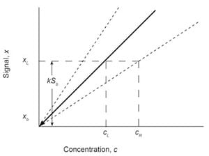
Fig. 7: Graphical approach to the LOD calculations using the analytical calibration curve of signal x and concentration c. The detection limit at reduced sensitivity cR is shown.
The ACS and EPA methodologies are not the only methods in use to calculate detection limits. A graphical approach is used that expresses the slope m as a confidence interval m ± taSm, where Sm is the standard deviation of the slope, and ta is a t-distribution value chosen for the desired confidence level a and the degrees of freedom v.5 Inserting this interval into Eq. (7) produces
cL = kSb/(m ± taSm) (12)
The effect of this inclusion is to bracket the slope of the analytical calibration curve with error bars that provide a maximum and minimum slope. These will provide detection levels for cL at reduced sensitivity cR and increased sensitivity. Generally, only the larger value of concentration cR is reported as the LOD. This can be shown graphically in Figure 7.
In an additional approach, the error in the intercept i, as well as the slope m, is considered. This method, the propagation of errors approach, considers the contribution of each term to the total error; a complete discussion of this method has appeared previously.5
Finally, instrumental detection limits (IDLs) are often used in the literature. They are provided by analysts who develop new or modified instrumentation for trace analysis.4 The IDLs are most often defined in terms of the standard deviation of measurements of the blank, usually with the value k = 2. The blank used is not a field blank containing some matrix but simply the solvent in which the sample is presented to the instrument. The IDLs have value when viewed as a rapid way of comparing instruments that are constantly evolving in their capability to detect trace amounts of analyte. Caution is needed with the use of IDLs. These limits in relation to practical analysis are unrealistically low. These results often cannot be matched in practical application outside the idealized laboratory setting.
Emerging EPA Methodologies
In late 1991, the EPA presented at the American Water Works Association Water Quality Technology Conference revised definitions of detection limits. These definitions, which are proposed to replace MDL and PQL, were first presented and discussed by Keith.27 PQLs have been criticized for lacking a strong technical basis because they are derived by the application of a multiplication factor to MDL.28 The main critical emphasis centers on the use of the word “limit” as a misnomer; the use of a 99% confidence level is inappropriate-higher confidence levels are required; the questions of false positives; and the use of zero as an arbitrary reference point.
The revised definitions for low-level analysis are method detection level (MDL’), reliable detection level (RDL), and reliable quantitation level (RQL). The intent of these definitions is to provide a consistent set of rules that reflect the operations necessary to provide realistic low-level analytical results for both regulators and those regulated. These definitions need to be broad to cover a large spectrum of environmental situations. It will also be advantageous to have a set of definitions that would receive broad acceptance within the scientific and regulatory community. The new definitions have been drafted so that they will provide clearer definitions with accompanying recommendations and accompanying usage guidance, and clearly interrelated terms. The proposed revisions to MDL’ will replace “limit” with “level,”; accommodate both zero and background signals of an analyte as a reference point, accommodate statistically variable confidence levels that may be used as a basis for estimating the probability of eliminating false-positive detections; take a representative matrix into consideration when making analytical measurements; and provide guidance on use and limitations of certainty in individual measurements.
The MDL’ is defined as follows:
The lowest concentration at which individual measurement results for a specific analyte are statistically different from a blank (that may be zero) with a specified confidence level for a given method and representative matrix. An interlaboratory MDL’ estimate represents the average detection capability of a single laboratory for a specific analyte method and matrix at a given point in time. An interlaboratory MDL’ estimate represents the method detection capability for a specific analyte and specific matrix determined in more than one laboratory.28
The RDL is defined as follows:
For a given MDL’, method, and representative matrix, a single analysis should consistently detect analytes present at concentrations equal to or greater than the RDL. When sufficient data are available, the RDL is the experimentally determined concentration at which false-negative and false-positive rates are specified. Otherwise, the RDL is the concentration that is twice that of the Method Detection Level (RDL = 2 x MDL’). The RDL is the recommended lowest level for qualitative decisions based on individual measurements, and it provides a much lower statistical probability of false-negative determinations than the MDL.28
The RQL is the recommended lowest level for quantitative decisions based on individual measurements for a given method and representative matrix. The RQL is the concentration that is two times the RDL (RQL = 2 x RDL). This recognizes that the RDL estimates produced at different times by different operators for different representative matrices will not often exceed the RQL.28
The EPA published these draft regulations in the June 1992 edition of the Federal Register. It is important to note that these are draft regulations and, as such, is subject to change; however, during an ACS-sponsored environmental symposium entitled, Regulatory Problems and Solutions with Method Detection Limits (April 6, 1992), there was overwhelming support for a change from the current MDL definition to those identified above.
Conclusion
As regulations develop in the present decade, the trend toward ever more stringent numerical standards is clear. Analytical variability, if not adequately understood and appropriately defined, can exacerbate the compliance obligation and regulatory burdens of both the regulator and regulated community. It is important for the metal-finishing industry to be knowledgeable as to the definition and application of detection-limit methodologies because they are becoming increasingly more common in its industrial regulations.
Article Written by John Lindstedt, CEO of Advanced Plating Technologies
References
- 1. “Nomenclature, Symbols, Units and Their Usage in Spectrochemical Analysis: II,” Spectrochemical Acta, 33B:242; 1978
- 2. MacDougal, D., et al., “Guidelines for Data Acquisition and Data Quality Evaluation in Environmental Chemistry,” Analytical Chemistry, 52:2242; 1980
- 3. “Detection Limits,” Analytical Chemistry, 58(9):986A; 1988
- 4. Thompson, M., et al., “Recommendations for the Definition, Estimation, and Use of the Detection Limit,” Analyst, 112:199-204; 1987
- 5. Long, G.L., and J.D. Winefordner, “Limit of Detection: A Closer Look at the IUPAC Definition,” Analytical Chemistry, 55(7):712A; 1983
- 6. Skoog, D.A. and D.W. West, “The Evaluation of the Reliability of Analytical Data.” In Fundamentals of Analytical Chemistry, 3rd Ed., Holt, Rinehart and Winston, New York, 1976, p. 59
- 7. Baumans, P.W.J.M, and F.J. de Boer, Spectrochemical Acta, 278:391; 1972
- 8. Glaser, J.A., et al., Environmental Science Technology, 15:1426; 1981
- 9. Baumans, P.W.J.M., Spectrochemical Acta, 338:625; 1978
- 10. Peters, D.G., et al., Chemical Separation and Measurements, WB Saunders, Philadelphia, 1974, Chapter 2
- 11. Baumans, P.W..M., Lines Coincidence Tables. Emission Spectrometry, Pergamon, Oxford; 1980
- 12. Currie. L.A., Analytical Chemistry, 40:586; 1968
- 13. Code of Federal Regulations, Vol.40, Appendix B to Part 136, Revision 1.11
- 14. Sotomayor, A., Keeping a Low Profile: Theoretical and Practical Considerations On Detection Limits, Office of Technical Services, Wisconsin Department of Natural Resources
- 15. Code of Federal Regulations, Vol. 40, Appendix A to Part 136 (1987)
- 16. Manual For Chemical Analysis of Water and Wastes, EPA 600/4-79-020, March 1983
- 17. Test Methods for Evaluating Solid Wastes, SW-846. November 1986. (Currently being revised: 54 Federal Register, 3212, January 23. 1989)
- 18. Federal Register, 52(130), No. 25,699; 1987
- 19. Department of the Army, U.S. Army Toxic and Hazardous Materials Agency; “Sampling and Chemical Analysis Assurance Program.” April 1982
- 20. Department of the Army, U.S. Army Toxic and Hazardous Materials Agency; “Installation Restoration Program. Quality Assurance Program,” December 1985
- 21. Gallo, D.P, et. al., “Written Comment on the Milwaukee Metropolitan Sewerage District’s Proposed Chapter 11 Rules,” August 12, 1991
- 22. Berthouex, P.M., “Much Ado About Next to Nothing-Judging Compliance At The Limit of Detection,” paper presented at 64th Annual Meeting of Centered States Water Pollution Control Association, May 14, 1991
- 23. Federal Register, Vol. 50, No. 46,906; 1985.
- 24. Federal Register, Vol. 50, No. 46902, p. 29; 1985.
- 25. Safe Water Drinking Act
- 26. Milwaukee Metropolitan Sewerage District Rules and Regulations, Chapter 11, Section 11.203 (l)(b), July I, 1992
- 27. Keith, L.H., “Documentation and Reporting,” Environmental Sampling and Analysis-A Practical Guide-, Lewis Publishers, 1991, pp.93-119
- 28. “Revising Definitions: Low-Level Analysis,” Environmental Lab, June/July, 58-61; 1992