Deposit Thickness in Surface Finishing
By: J. Lindstedt, President. ![]()
In ordering a surface coating system to enhance the performance of an article in service, the use of standard finishing specifications is the established procedure employed by most manufacturing entities. The specifications most commonly referenced are ASTM, MIL Specs, AMS and unique corporate specifications.
Surface finishing specifications identify a number of parameters which evaluate the ability of the surface coating to perform its intended function. The most common coating requirements used to qualify a coating system are:
- Deposit thickness: This parameter is often defined by a service class. Service class prescribes a deposit thickness as a function of intended use. Service classes are easily found in most ASTM specifications.Thickness is defined by several definitions, minimum, maximum, average and average range.
- Deposit appearance: The appearance description is a generic narrative of the visual attributes of the applied coating.
- Deposit adhesion: This parameter is defined by several methodologies. Most of these criteria will stress the coating/basis metal interface in an attempt to remove the deposit from the basis metal. These tests typically stress the coating metallurgical bond by mechanical or thermal means. The prevalent standard tests are found in ASTM B571.
- Penultimate plating requirements: Often the coating system selected is a series of deposits to provide the required performance. This section will define the additional deposits below the final deposit, order of application and required thickness of any penultimate layer.
- Secondary performance prerequisites: These additional testing protocols are most typically hydrogen embrittlement relief, solderability and accelerated corrosion testing.
Of all of these parameters the one which is the least understood and thus often incorrectly applied is deposit thickness. Unfortunately, this leads to confusion and the frequent over or under application of deposit thickness which results in needless delays in securing acceptable components.
Understanding Deposit Thickness Variation
Deposits as applied by electrolytic or electroless methodologies by barrel, rack or continuous strip plating techniques will all be normally distributed as defined by the Gaussian distribution curve. The distribution curve of deposit thickness is defined as a function of x(thickness) in Equation 1 below:
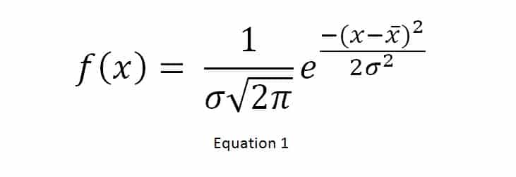
where:
x is the sample measurement i.e. deposit thickness
x-bar is the arithmetic mean of x data points
σ is the population standard deviation
This function is shown graphically as
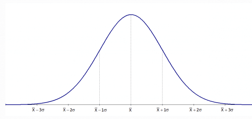
Figure 1: Normal Gaussian Distribution Curve
In this graph it is clear that the thickness of a deposit at a single measurement location is not a single repeatable value but a distribution of numbers that cluster about a central value, the arithmetic mean, and the variation about that central value is defined by the standard deviation. The standard deviation is a measure used to quantify the variation or dispersion of a set of data values. The standard deviation is defined in Equation 2.
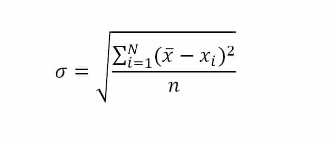
Equation 2: Standard Deviation of Population
where:
x is the sample measurement i.e. deposit thickness
x-bar is the arithmetic mean of x data points
σ is the population standard deviation
n is the number of data points
It is key to an understanding of deposit thickness on an article at a single measurement location is that it is not a single repeatable data point but a scattering of values that will accumulate around a central tendency, the arithmetic mean.
The breadth or width of the dispersion is defined by the variation of the process. It is the width of the dispersion that must be considered when designing an article. It is this variation in thickness that will impact mechanical fit of components, corrosion performance, solderabiliy etc. It is also critical to consider the process variation when defining quality acceptance criteria.
The percentage of data points that cluster about the arithmetic mean can be calculated by the techniques of integral calculus where the area under the curve is computed. Thus the area under the curve from plus infinity(+∞) to minus infinity(-∞) represents 100% of all data points in the distribution. The area under the left hand portion of the curve from -∞ to the mean represents 50% of all data points. The same is true for the right hand portion of the area from +∞ to the mean.
Similarly, any area between any two values of the x axis can be calculated and the area divided by the total area to calculate the percent of measurements that are contained between the two selected points. The percentage of data points in a normal distribution that exit between -1σ and +1σ is 68.26%. The data points that exist between -2σ and +2σ standard deviations is 95.44%, and similarly the data points that exist between -3σ and +3σ is 98.74%. This is shown in Figure 2 below.
Figure 2: Percentage of Data Points between +/- 1, 2 or 3 Standard Deviations
From Figure 2 several facts regarding the standard deviation of a process are evident.
- The absolute value of the standard deviation is an important parameter to use in defining the range of thickness values which are to be expected from a surface finishing process. To completely define the thickness of a deposit on an article, thought must be given to the dispersion of data points. As the magnitude of the standard deviation increases the dispersion of data increases thus resulting in deposit thickness data points that can be very small or very large. Thus, fewer data points cluster about the central tendency and the range of deposit thickness increases. This has design considerations that need to be addressed.
Example:
If a process has a large standard deviation, special consideration in the use of maximum or minimum specifications must be evaluated. For example, if a supplier specifies a minimum specification which is defined as NO values below the stated thickness and there is a quality acceptance criteria of 2000 ppm (0.2% defective), this will force a supplier to select a targeted average deposit thickness that is at least 4 standard deviations greater than the specified minimum thickness such that no values are measured below the specified minimum value. This will have dramatic size implications on those data points that are in the right hand portion of the distribution curve. This resultant number of thickness values that are greater than the elevated target average thickness may be an issue as there will be articles measured at the mean plus 4 standard deviations. These data points certainly need to be considered in the use of the stated mimimum specification.
- At +/- 3σ there still exits 0.26% of values that are significantly less than the mean or significantly greater than the mean. This has large implications in corrosion performance or in sizing concerns if a quality acceptance level of less than 2600 ppm (0.26% defective) is the requirement. While this represents a small percentage of product,0.26%, this level of unacceptable product is often an issue in the automotive, medical or aerospace industries.
Modification of the Magnitude of the Standard Deviation
As shown above, deposit thickness in surface finishing is composed of two main elements, the arithmetic mean and the dispersion of that data about the mean, the standard deviation. Clearly it is critical to minimize the size of the standard deviation to more closely cluster as much data as possible about the central tendency. This provides a much more consistent and homogeneous thickness data set which facilitates product design and quality compliance.
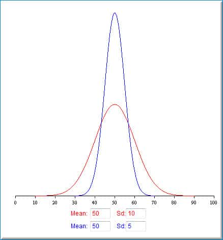
Figure 3: Demonstration of Strong and Weak Central Tendency of Data Sets
Figure 3 demonstrates the variation in data with a standard deviation 50 % smaller than an alternate example. In the red data set 95% of the data will reside between 30 and 70 units. In the blue data set 95% of the data will reside between 40 and 60 units. If the parameter of concern is dimensional and the graph depicts deposit thickness the smaller tighter variance would be of value in providing a much more uniform and consistent article for fit and function. A similar discussion would follow if corrosion testing where of concern. The tighter grouped data of thickness would provide a more corrosion resistant product with many fewer articles at reduced thickess of less than or equal to 25 and thus reduced occurance of corrosion failures.
Reducing the Spread of Thickness Data – Electroless versus Electrolytic
The plating process can be selected and modified to reduce the magnitude of the standard deviation. All deposition processes either electrolytic or electroless are normally distributed with the electrolytic methodology having an intrinsically greater standard deviation than electroless plating processes. Therefore the first decision for a design engineer to make is to select an electroless process over an electrolytic one if there is a need to reduce the spread or range of deposit thickness. If that decision is not possible i.e. an electroless process is not available for the metal required then other choices need to be made.
The following choices will reduce the standard deviation for electrolytic deposition systems.
- Selection of a plating system that deposits from a complexed cation versus a simple ion. An example of this would be to copper plate from a cyanide electrolyte rather than an acid matrix.
- Reducing the current density used during processing.
- Use of a barrel plating technique versus a rack plating technique.
- If rack plating, the employment of shields will reduce standard deviation.
- Operation of the chemical system at the low end of operational temperature range.
- In barrel plating, techniques that enhance mixing i.e. barrel rotational speed, serrated barrel cylinder walls, breaker bars will assist in obtaining lower standard deviations.
- Maintaining solution chemistry within 2% of optimal.
The following choices will reduce the standard deviation for electroless deposition systems.
- In rack plating, use of enhanced solution mixing i.e. proper air flow, use of cathode bar agitation or both simultaneously.
- In barrel plating, techniques that enhance mixing i.e. barrel rotational speed, serrated barrel cylinder walls, breaker bars will assist in obtaining lower deviations.
- Maintaining solution chemistry within 2% of optimal